
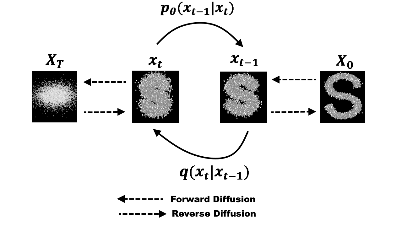
Let $X_0$ the input image, the goal of the diffusion process is to gradually add noise to the image until its pixel values approximate a standard normal distribution. This enables a neural network to be trained to reverse the diffusion process and reconstruct the original image from the noised image. In this post, we will focus on the mathematical details behind the noise injection step of the diffusion process. The single step of injecting noise can be defined as follows:
$$X_t \sim N( \sqrt{1 - \beta_t} X_{t-1}, \beta_t \mathbf{I}) $$where $\beta_t$ is the fixed variance of the Gaussian distribution at time $t$. The variance of the diffusion process is defined to be strictly increasing with time, i.e. $\beta_1 < \beta_2 ... < \beta_T $.
We can compute the value of $X_t$ by sampling from its distribution. However, to do it in a differentiable way, we can use the reparametrization trick as follows:
$$ X_t =\sqrt{1 - \beta_t} X_{t-1} + \sqrt{\beta_t} \epsilon_t $$where $\epsilon_t \sim N(0, \mathbf{I})$. As in the original paper, we can reparametrize $\beta_t$ as $\alpha_t = 1 - \beta_t $ and therefore rewrite the latter equation as
$$ X_t =\sqrt{\alpha_t} X_{t-1} + \sqrt{1 - \alpha_t} \epsilon_t $$Now, let’s go deeper and write $X_t$ as a function of $X_{t-2}$:
$$ \begin{align*} X_t & = \sqrt{\alpha_t} X_{t-1} + \sqrt{1 - \alpha_t} \epsilon_t \\\\ & = \sqrt{\alpha_t} (\sqrt{\alpha_{t-1}} X_{t-2} + \sqrt{1 - \alpha_{t-1}} \epsilon_{t-1}) + \sqrt{1 - \alpha_t} \epsilon_t \\\\ & = \sqrt{\alpha_t \alpha_{t-1}} X_{t-2} + \underbrace{\sqrt{\alpha_t (1 - \alpha_{t-1})} \epsilon_{t-1}}\_{N(\mathbf{0}, \sqrt{\alpha_t (1 - \alpha_{t-1})} \mathbf{I})} + \underbrace{\sqrt{1 - \alpha_t} \epsilon_t}\_{N(\mathbf{0}, \sqrt{1 - \alpha_t} \mathbf{I})} \\\\ & = \sqrt{\alpha_t \alpha_{t-1}} X_{t-2} + \sqrt{\alpha_t (1 - \alpha_{t-1}) + (1 - \alpha_t)} \hat{\epsilon_{t-1}} \\\\ & = \sqrt{\alpha_t \alpha_{t-1}} X_{t-2} + \sqrt{1 - \alpha_t \alpha_{t-1}} \hat{\epsilon_{t-1}} \end{align*} $$where $\hat{\epsilon_{t-1}} \sim N(\mathbf{0}, \mathbf{I})$. In the last step of the equation above, we have used the fact that the sum of two independent Gaussian random variables is also a Gaussian random variable with mean equal to the sum of the means and variance equal to the sum of the variances, i.e. $N(\mu_1, \sigma_1^2) + N(\mu_2, \sigma_2^2) = N(\mu_1 + \mu_2, \sigma_1^2 + \sigma_2^2)$. Finally, we can continue this process until we reach $X_0$:
$$ \begin{align*} X_t & = \sqrt{\alpha_t} X_{t-1} + \sqrt{1 - \alpha_t} \epsilon_t \\\\ & = \sqrt{\alpha_t \alpha_{t-1} \dots \alpha_1} X_0 + \sqrt{ (1 - \alpha_t \alpha_{t-1} \dots \alpha_1)} \hat{\epsilon_{t-1}} \end{align*} $$Let $\overline{\alpha_t} = \alpha_t \alpha_{t-1} \dots \alpha_1$ then we can rewrite the latter equation as follows:
$$ X_t = \sqrt{\overline{\alpha_t}} X_0 + \sqrt{1 - \overline{\alpha_t}} \hat{\epsilon_{t-1}} $$