Technical notes on MuLAN

MuLAN

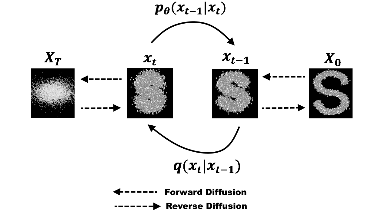
MuLAN by Sahoo et al. (2024) is a diffusion model built on top of Variational Diffusion Models that achieves SOTA on likelihood estimation on image datasets with the following features:

• Multivariate noising schedule (i.e. every timestep has a different noise rate)
• The noising schedule is described by a 5-degree polinomial
• Noising schedule is conditioned on a latent discrete variable, dependent on the input

In these notes I tried to summarize the most important technical parts of MuLAN

MuLAN Algorithms

Training Algorithm

The MuLAN training procedure optimizes both the denoising model parameters $\theta$ and encoder/noise schedule parameters $\phi$ jointly:

Repeat until convergence:

1. Sample a data point $\mathbf{x} _ 0$ from the dataset $q(\mathbf{x} _ 0)$
2. Encode $\mathbf{x} _ 0$ to get the distribution for the auxiliary latent variable, then sample $\mathbf{z} \sim q _ \phi(\mathbf{z}|\mathbf{x} _ 0)$
3. Sample a random time $t \sim U[0, 1]$ and a random noise vector $\boldsymbol{\epsilon} \sim \mathcal{N}(\mathbf{0}, \mathbf{I})$
4. Compute the multivariate noise schedule $\boldsymbol{\gamma} _ \phi(\mathbf{z}, t)$ using the learned schedule network
5. Compute schedule parameters: $\boldsymbol{\alpha} _ t(\mathbf{z}) = \sqrt{\text{sigmoid}(-\boldsymbol{\gamma} _ \phi(\mathbf{z}, t))}$ and $\boldsymbol{\sigma} _ t(\mathbf{z}) = \sqrt{\text{sigmoid}(\boldsymbol{\gamma} _ \phi(\mathbf{z}, t))}$
6. Create the noised sample: $\mathbf{x} _ t = \boldsymbol{\alpha} _ t(\mathbf{z})\mathbf{x} _ 0 + \boldsymbol{\sigma} _ t(\mathbf{z})\boldsymbol{\epsilon}$
7. Predict the noise $\boldsymbol{\epsilon} _ \theta(\mathbf{x} _ t, \mathbf{z}, t)$ using the U-Net model
8. Compute the total loss $\mathcal{L}$ based on the Evidence Lower Bound (ELBO): $\mathcal{L} = \mathcal{L} _ \text{recons} + \mathcal{L} _ \text{diffusion} + \mathcal{L} _ \text{prior} + \mathcal{L} _ \text{latent}$
9. Compute gradients $\nabla _ {\theta, \phi} \mathcal{L}$ and update parameters $\theta$ and $\phi$ with an optimizer step

Generation Algorithm (Sampling)

Given trained model parameters $\theta$ and $\phi$ :

1. Sample an auxiliary latent variable from the prior: $\mathbf{z} \sim p _ \theta(\mathbf{z})$

2. Sample an initial state from the noise distribution: $\mathbf{x} _ 1 \sim \mathcal{N}(\mathbf{0}, \mathbf{I})$

3. Define the reverse probability flow ODE:

   $$\frac{d\mathbf{x} _ t}{dt} = \mathbf{h} _ \theta(\mathbf{x} _ t, \mathbf{z}, t) = \left[ \mathbf{f}(\mathbf{z}, t)\mathbf{x} _ t - \frac{1}{2}\mathbf{g}^2(\mathbf{z}, t) \mathbf{s} _ \theta(\mathbf{x} _ t, \mathbf{z}, t) \right]$$

   where the drift $\mathbf{f}$ and diffusion $\mathbf{g}$ are derived directly from the learned noise schedule $\boldsymbol{\gamma} _ \phi$ :

   • $\mathbf{g}^2(\mathbf{z}, t) = \text{sigmoid}(\boldsymbol{\gamma} _ \phi(\mathbf{z}, t)) \cdot \nabla _ t\boldsymbol{\gamma} _ \phi(\mathbf{z}, t)$
   • $\mathbf{f}(\mathbf{z}, t) = -\frac{1}{2}\mathbf{g}^2(\mathbf{z}, t)$ The term $\mathbf{s} _ \theta(\mathbf{x} _ t, \mathbf{z}, t)$ is the score function, approximated by the trained U-Net. For noise parameterization: $\mathbf{s} _ \theta(\mathbf{x} _ t, \mathbf{z}, t) = -\frac{\boldsymbol{\epsilon} _ \theta(\mathbf{x} _ t, \mathbf{z}, t)}{\boldsymbol{\sigma} _ t(\mathbf{z})}$

4. Numerically solve the ODE from $t=1$ down to $t=0$ using a solver (e.g., RK45) with initial condition $\mathbf{x} _ 1$

5. The result of the integration at $t=0$ is the generated sample $\mathbf{x} _ 0$

Technical Details

The training objective of MuLAN is to maximize the Evidence Lower Bound (ELBO) on the log-likelihood of the data:

This objective is optimized end-to-end, jointly training all model components.

Loss Function Components

The total loss is a sum of four distinct terms, each with a specific role:

Diffusion Loss ( $\mathcal{L} _ \text{diffusion}$ ): This is the core term that drives the learning of the denoising model and the noise schedule. It is computed as the weighted squared error between the true noise and the predicted noise, sampled at a random time $t$ . Its continuous-time form is:

The weighting by $\nabla _ t \boldsymbol{\gamma} _ \phi(\mathbf{z}, t)$ , the gradient of the learned noise schedule, is what makes the ELBO path-dependent and allows for the optimization of the noising process itself.

Reconstruction Loss ( $\mathcal{L} _ \text{recons}$ ): This term corresponds to the likelihood of reconstructing the original data $\mathbf{x} _ 0$ from the first denoising step. It is the negative log-likelihood of the decoder at the first timestep: $-\log p _ \theta(\mathbf{x} _ 0 | \mathbf{z}, \mathbf{x} _ 1)$ .

Prior Matching Loss ( $\mathcal{L} _ \text{prior}$ ): This term ensures that the distribution of the fully noised data $q(\mathbf{x} _ 1 | \mathbf{x} _ 0, \mathbf{z})$ matches a simple, fixed prior distribution $p _ \theta(\mathbf{x} _ 1)$ (typically a standard normal distribution). It is a KL divergence term: $\text{KL}[q(\mathbf{x} _ 1| \mathbf{x} _ 0, \mathbf{z}) \| p _ \theta(\mathbf{x} _ 1)]$ .

Latent Regularization Loss ( $\mathcal{L} _ \text{latent}$ ): This term regularizes the encoder $q _ \phi(\mathbf{z}|\mathbf{x} _ 0)$ by encouraging the distribution of the auxiliary latent $\mathbf{z}$ to match a simple prior $p _ \theta(\mathbf{z})$ . It is also a KL divergence: $\text{KL}[q _ \phi(\mathbf{z}|\mathbf{x} _ 0) \| p _ \theta(\mathbf{z})]$ . Depending on whether $\mathbf{z}$ is continuous or discrete, this term is computed as a standard Gaussian KL divergence or a KL divergence between categorical distributions.

Obtaining the Learned Adaptive Noise Schedule

The noise schedule $\boldsymbol{\gamma} _ \phi(\mathbf{z}, t)$ is not handcrafted but is instead the output of a neural network parameterized by $\phi$ . The paper proposes a novel polynomial parameterization for its superior performance and desirable properties.

1. A small MLP, also part of the parameters $\phi$ , takes the latent context $\mathbf{z}$ as input and outputs three coefficient vectors: $\mathbf{a}(\mathbf{z}), \mathbf{b}(\mathbf{z}), \mathbf{d}(\mathbf{z})$

2. These coefficients are used to construct a monotonic degree-5 polynomial function of time $t$ , $f _ \phi(\mathbf{z}, t)$ :

   $$f _ \phi(\mathbf{z}, t) = \frac{\mathbf{a}^2(\mathbf{z})}{5} t^5 + \frac{\mathbf{a}(\mathbf{z})\mathbf{b}(\mathbf{z})}{2}t^4 + \frac{\mathbf{b}^2(\mathbf{z}) + 2\mathbf{a}(\mathbf{z})\mathbf{d}(\mathbf{z})}{3} t^3 + \mathbf{b}(\mathbf{z})\mathbf{d}(\mathbf{z}) t^2 + \mathbf{d}^2(\mathbf{z})t$$

   All operations are element-wise. This construction guarantees that the function is monotonically increasing with respect to $t$ .

3. The final schedule $\boldsymbol{\gamma} _ \phi(\mathbf{z}, t)$ is obtained by scaling this polynomial to lie within a predefined range $[\gamma _ \text{min}, \gamma _ \text{max}]$ :

   $$\boldsymbol{\gamma} _ \phi(\mathbf{z}, t) = \gamma _ \text{min} + (\gamma _ \text{max} - \gamma _ \text{min}) \frac{f _ \phi(\mathbf{z}, t)}{f _ \phi(\mathbf{z}, t=1)}$$

   This ensures that the diffusion process starts and ends at fixed noise levels while the path between them is learned.