Diffusion models are the state of the art in terms of generative models and I wanted to contribute in my own way with a self-complete article that summarizes the diffusion model training and sampling.
We define first some common terminology, then we describe the training and sampling process. Finally we define the most common ODE samplers used for generating data and we focus on the Classifier-Free guidance.
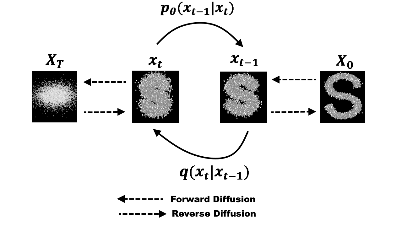
In this article we assume intuitive understand of what a generative model and what a diffusion models does (inject noise, denoise). We adopt the Variational Diffusion Model (VDM) formulation. To describe the noising process we adopt the convention
$$ t = 0 \;\Rightarrow\; x_0\; \text{clean sample}, \qquad t = 1 \;\Rightarrow\; x_1\; \text{pure noise} \sim \mathcal{N}(\mathbf{0}, \mathbf{I}). $$So $t$ runs forward from data to noise during the diffusion process, and the model’s job will be to run it backward.
Training a diffusion model means teaching a network parametrized by $\theta$ to predict the noise that was added at an arbitrary point along this schedule. Concretely, each training step does three things.
1. Sample a timestep.
$$ t \sim \mathcal{U}[0,1]. $$2. Inject noise. Given the clean sample $x_0$, we form the noisy sample
$$ x_t = \alpha_t\, x_0 + \sigma_t\, \boldsymbol{\varepsilon}, \qquad \boldsymbol{\varepsilon} \sim \mathcal{N}(0, I), $$where the signal and noise coefficients $\alpha_t$ and $\sigma_t$ come straight from the schedule:
$$ \alpha_t = \sqrt{\operatorname{sigmoid}\big(-\gamma(t)\big)}, \qquad \sigma_t = \sqrt{\operatorname{sigmoid}\big(\gamma(t)\big)}. $$We can see how both terms are determined by $\gamma(\cdot)$, which is the log Signal-to-Noise ratio. Down below we will describe how the noise schedule $\gamma(\cdot)$ can be defined.
3. Predict the noise. The network outputs $\boldsymbol{\varepsilon}_\theta(x_t, t, c)$, an estimate of the $\boldsymbol{\varepsilon}$ we just added, optionally conditioned on a context vector $c$ (see Classifier-Free Guidance).
Noise Schedule. The schedule $\gamma_t$ itself can take several forms. Once the endpoints $\gamma_0$ and $\gamma_1$ are fixed, the common choices are:
$$\begin{aligned} \text{Linear:} &\quad \gamma_0 + (\gamma_1 - \gamma_0)\, t, \\ \text{Cosine:} &\quad \gamma_0 + (\gamma_1 - \gamma_0)\, \tfrac{1}{2}\big(1 - \cos(\pi t)\big), \\ \text{Learned:} &\quad \gamma_0 + (\gamma_1 - \gamma_0)\, \mathrm{MLP}_\eta(t), \\ \text{Multivariate Learned:} &\quad \gamma_0 + (\gamma_1 - \gamma_0)\, \mathbf{MLP}_\eta(t, c), \end{aligned}$$where $\mathrm{MLP}(t)$ is a positive monotonic network, i.e.
$$ t_1 > t_2 \;\Longrightarrow\; \mathrm{MLP}(t_1) > \mathrm{MLP}(t_2). $$We can go one step further with a multivariate learned contextual schedule: part of $\gamma$ is fixed and learned globally, while another part is estimated from the context $c$, letting the noise schedule adapt to the input.
With predictions in hand, the loss combines three terms:
$$ \begin{aligned} \text{1. Standard diffusion loss:}\quad & \big\| \boldsymbol{\varepsilon} - \hat{\boldsymbol{\varepsilon}}_\theta(x_t, t, c) \big\|, \\[2pt] \text{2. Reconstruction loss:}\quad & \big\| \boldsymbol{\varepsilon} - \boldsymbol{\varepsilon}_\theta(x_{0+s}, \Delta, c) \big\|, \qquad s \to 0^{+}, \\[2pt] \text{3. Prior loss:}\quad & \big\| \boldsymbol{\varepsilon} - \boldsymbol{\varepsilon}_\theta(x_1, I, c) \big\|. \end{aligned} $$The first term is the usual denoising objective. The last two terms anchor the endpoints of the process and, in our experience, are particularly useful when the noise schedule itself is being learned.
Once the network is trained, how do we turn pure noise back into data? That is the sampling problem.
We develop two types of sampling: ancestral sampling and ODE sampling. While the first relies partially on stochastic variables, the second is purely deterministic.
To sample with the VDM we walk the schedule backward, drawing from the conditional distribution $p(x_s \mid x_t)$ with $s < t$:
$$ p(z_s \mid z_t) = \mathcal{N}\!\big(\boldsymbol{\mu}_\theta(z_t; s, t),\; \sigma_Q^2(s,t)\, \boldsymbol{I}\big), $$with
$$ \begin{aligned} \boldsymbol{\mu}_\theta(z_t; s, t) &= \frac{\alpha_s}{\alpha_t} \Big(z_t + \sigma_t\, \operatorname{expm1}\!\big(\gamma_\eta(s) - \gamma_\eta(t)\big)\, \boldsymbol{\varepsilon}_\theta(z_t; t)\Big), \\[4pt] \sigma_Q^2(s,t) &= \sigma_s^2\Big(-\operatorname{expm1}\!\big(\gamma_\eta(s) - \gamma_\eta(t)\big)\Big), \end{aligned} $$where $\operatorname{expm1}(\cdot) := \exp(\cdot) - 1$. Equivalently, a single ancestral step can be written explicitly as
$$ z_s = \sqrt{\frac{\sigma_s^2}{\sigma_t^2}} \underbrace{\Big(z_t - \sigma_t \big(-\operatorname{expm1}(\gamma_\eta(s) - \gamma_\eta(t))\big)\, \boldsymbol{\varepsilon}_\theta(z_t; t)\Big)}_{\text{deterministic part}} + \underbrace{\sqrt{(1 - \alpha_s^2) \big(-\operatorname{expm1}(\gamma_\eta(s) - \gamma_\eta(t))\big)}\;\boldsymbol{\varepsilon}}_{\text{stochastic part}}, $$with $\boldsymbol{\varepsilon} \sim \mathcal{N}(0,1)$. The first bracket pulls the sample toward the denoised estimate; the second injects fresh noise.
The stochastic sampler is simple but tends to need many steps. If we are willing to drop the noise injection, we can instead describe the reverse process as a deterministic ODE, which opens the door to fast, high-order numerical solvers.
Every diffusion process has an associated forward SDE of the form
$$ dx = f(x, t)\, dt + g(t)\, d\boldsymbol{w}, $$and a corresponding probability-flow ODE that shares the same marginals but is fully deterministic:
$$ \frac{dx}{dt} = f(x, t) - \tfrac{1}{2}\, g(t)^2\, \nabla_{x} \log p_t(x). $$In VDM we adapt the terms $f(x, t)$ and $g(t)$ as follows:
$$ \begin{aligned} f(x, t) &= \frac{d \log \alpha_t}{dt}\, x, \\[4pt] g(t)^2 &= \frac{d \sigma_t^2}{dt} - 2\,\frac{d \log \alpha_t}{dt}\, \sigma_t^2. \end{aligned} $$In other words, the VDM drift $f(x,t)$ is just a time-dependent scaling of the current state, and the diffusion coefficient $g(t)$ measures how fast variance is being pumped in net of that scaling. The only learned object is the score $\nabla_{x} \log p_t(x)$, which we read off directly from the noise prediction:
$$ \nabla_{x} \log p_t(x) \approx -\frac{\boldsymbol{\varepsilon}_\theta(x, t)}{\sigma_t}. $$Substituting these into the probability-flow ODE gives a closed-form vector field that depends only on the schedule and the network output, which is exactly the function $f(t_m, z_m, \theta)$ that the solvers below will integrate.
Continuous-time diffusion models formulate the generative process $\boldsymbol{x}_1 \to \boldsymbol{x}_0$ over a continuous time domain $t \in [0, 1]$ as the path of a Stochastic Differential Equation (SDE). By mapping this SDE to an equivalent deterministic Probability-Flow Ordinary Differential Equation (ODE), we cast the generative model as a Continuous Normalizing Flow (CNF). This permits exact likelihood estimation $\log p_\theta(\boldsymbol{x}_0)$ via the instantaneous change-of-variables theorem.
Let $\boldsymbol{x}_0 \sim p_{\text{data}}(\boldsymbol{x}_0)$ be a sample from the underlying data manifold. The forward diffusion process corrupts $\boldsymbol{x}_0$ progressively over $t \in [0, 1]$ to yield noised latents $\boldsymbol{x}_t \in \mathbb{R}^d$, governed by the Gaussian transition kernel:
$$ q(\boldsymbol{x}_t \mid \boldsymbol{x}_0) = \mathcal{N}(\boldsymbol{x}_t; \alpha_t \boldsymbol{x}_0, \sigma_t^2 \boldsymbol{I}). $$Equivalently, this forward dynamic maps exactly to the solution of the linear It^o SDE:
$$ d\boldsymbol{x}_t = \boldsymbol{f}(\boldsymbol{x}_t, t)\, dt + g(t)\, d\boldsymbol{w}_t, $$where $\boldsymbol{w}_t$ is the standard forward Wiener process. In the VDM parameter space, the drift vector field $\boldsymbol{f}(\boldsymbol{x}_t, t)$ and the scalar diffusion coefficient $g(t)$ expand analytically as:
$$ \boldsymbol{f}(\boldsymbol{x}_t, t) = \left( \frac{d}{dt} \log \alpha_t \right)\boldsymbol{x}_t, \qquad g(t) = \sqrt{\frac{d}{dt}\sigma_t^2 - 2\sigma_t^2\, \frac{d}{dt}\log \alpha_t}. $$Following Anderson’s theorem, the reverse-time generation—flowing from $t=1$ back to $t=0$—is characterized by a corresponding reverse SDE:
$$ d\boldsymbol{x}_t = \left[\boldsymbol{f}(\boldsymbol{x}_t, t) - g(t)^2\, \nabla_{\boldsymbol{x}_t} \log p_t(\boldsymbol{x}_t)\right]dt + g(t)\, d\bar{\boldsymbol{w}}_t, $$where $\bar{\boldsymbol{w}}_t$ denotes a reverse-time Wiener process, and $\nabla_{\boldsymbol{x}_t} \log p_t(\boldsymbol{x}_t)$ is the Stein score of the marginal density $p_t(\boldsymbol{x}_t)$. Crucially, Song et al. (2021) demonstrated that there exists a deterministic probability-flow ODE sharing the identical marginal probability densities $\{p_t(\boldsymbol{x}_t)\}_{t \in [0, 1]}$ as the SDE:
$$ d\boldsymbol{x}_t = \underbrace{\left[ \boldsymbol{f}(\boldsymbol{x}_t, t) - \tfrac{1}{2} g(t)^2\, \nabla_{\boldsymbol{x}_t} \log p_t(\boldsymbol{x}_t) \right]}_{\widetilde{\boldsymbol{f}}(\boldsymbol{x}_t, t)} dt. $$In practice, the exact score $\nabla_{\boldsymbol{x}_t} \log p_t(\boldsymbol{x}_t)$ is intractable. We approximate it using our neural network via the standard score-to-noise parameterization, creating our parameterized ODE drift field $\widetilde{\boldsymbol{f}}_\theta(\boldsymbol{x}_t, t)$.
Because this ODE describes a continuous normalizing flow mapping the known prior $p_1(\boldsymbol{x}_1) \approx \mathcal{N}(\boldsymbol{0}, \boldsymbol{I})$ to the complex targeted distribution $p_\theta(\boldsymbol{x}_0)$, we can invoke the instantaneous change-of-variables formula from Neural ODEs (Chen et al., 2018) to compute the exact log-likelihood:
$$ \log p_\theta(\boldsymbol{x}_0) = \log p_1(\boldsymbol{x}_1) - \int_0^1 \nabla_{\boldsymbol{x}_t} \cdot \widetilde{\boldsymbol{f}}_\theta(\boldsymbol{x}_t, t)\, dt, $$where the divergence operator $\nabla_{\boldsymbol{x}_t} \cdot \widetilde{\boldsymbol{f}}_\theta(\boldsymbol{x}_t, t) \equiv \operatorname{tr}\!\left(\nabla_{\boldsymbol{x}_t} \widetilde{\boldsymbol{f}}_\theta(\boldsymbol{x}_t, t)\right)$ acts as the infinitesimal volume expansion term, and the parameterized field defines as:
$$ \widetilde{\boldsymbol{f}}_\theta(\boldsymbol{x}_t, t) := \boldsymbol{f}(\boldsymbol{x}_t, t) - \tfrac{1}{2} g(t)^2\, \boldsymbol{\epsilon}_\theta(\boldsymbol{x}_t, t). $$Consequently, evaluating the exact likelihood condenses down to integrating the divergence of the neural ODE drift field continuously tracked along the generated trajectory.
Directly computing $\operatorname{tr}(\nabla_{\boldsymbol{x}_t} \tilde{f}_\theta)$ requires a full Jacobian and scales as $\mathcal{O}(d^2)$. To avoid this, we use Hutchinson’s estimator. For any matrix $\boldsymbol{A} \in \mathbb{R}^{d\times d}$,
$$ \operatorname{tr}(\boldsymbol{A}) = \mathbb{E}_{\boldsymbol{v}}[\boldsymbol{v}^\top \boldsymbol{A}\, \boldsymbol{v}], $$if $\mathbb{E}[\boldsymbol{v}] = \boldsymbol{0}$ and $\mathbb{E}[\boldsymbol{v}\boldsymbol{v}^\top] = \boldsymbol{I}$.
To see unbiasedness, expand
$$ \boldsymbol{v}^\top \boldsymbol{A}\, \boldsymbol{v} = \sum_{i=1}^d\sum_{j=1}^d v_i A_{ij} v_j. $$Taking expectation,
$$ \mathbb{E}[\boldsymbol{v}^\top \boldsymbol{A}\, \boldsymbol{v}] = \sum_{i=1}^d\sum_{j=1}^d A_{ij}\, \mathbb{E}[v_i v_j]. $$Because $\mathbb{E}[v_i v_j] = \delta_{ij}$, we obtain
$$ \mathbb{E}[\boldsymbol{v}^\top \boldsymbol{A}\, \boldsymbol{v}] = \sum_{i=1}^d A_{ii} = \operatorname{tr}(\boldsymbol{A}). $$In diffusion likelihood estimation this is crucial: we never materialize the full Jacobian, and instead compute Jacobian-vector products, reducing practical cost from quadratic to roughly linear in dimension per probe. In practice, averaging a small number of probes (often around $5$-$10$) is already effective.
The projection vector $\boldsymbol{v} \in \mathbb{R}^d$ must satisfy
$$ \mathbb{E}[\boldsymbol{v}] = \boldsymbol{0}, \qquad \mathbb{E}[\boldsymbol{v}\boldsymbol{v}^\top] = \boldsymbol{I}. $$Two common choices are:
Both satisfy the required moment conditions and therefore produce unbiased trace estimates.
Terminology. Given a step size $h$, we want to advance from timestep $t_m$ to $t_{m+1}$ starting from our sample $z_m$, where $f(\cdot)$ denotes the ODE vector field derived above. The different solvers below trade off accuracy against the number of function evaluations (NFE).
While computationally inexpensive, this first-order method accumulates local errors on the order of $\mathcal{O}(h^2)$, at a cost of $1$ NFE per step.
A second-order Runge–Kutta method that estimates the vector field at the midpoint of the integration step, giving a more accurate gradient estimate:
$$ \begin{aligned} k_1 &:= f(t_m, z_m, \theta), \\ k_2 &:= f\!\Big(t_m + \tfrac{h}{2},\; z_m + \tfrac{h}{2} k_1,\; \theta\Big), \\ z_{m+1} &= z_m + h\, k_2. \end{aligned} $$Error: $\mathcal{O}(h^3)$, at $2$ NFE.
Pushing the same idea further, RK4 blends four slope evaluations:
$$ \begin{aligned} k_1 &= f(t_m, z_m, \theta), \\ k_2 &= f\!\Big(t_m + \tfrac{h}{2},\; z_m + \tfrac{h}{2} k_1,\; \theta\Big), \\ k_3 &= f\!\Big(t_m + \tfrac{h}{2},\; z_m + \tfrac{h}{2} k_2,\; \theta\Big), \\ k_4 &= f\big(t_m + h,\; z_m + h\, k_3,\; \theta\big), \\ z_{m+1} &= z_m + \tfrac{h}{6}\big(k_1 + 2k_2 + 2k_3 + k_4\big). \end{aligned} $$Error: $\mathcal{O}(h^5)$, at $4$ NFE.
So far every method uses a fixed step size. The smarter move is to let the solver pick $h$ on the fly based on how hard the trajectory is to integrate — this is what adaptive solvers do.
This method is adaptive: the NFE depends on the local approximation error. The trick is to compute two Runge–Kutta solutions of different order (5th and 4th) from the same stages and use their difference as an error estimate. The stages are
$$ k_i = f\!\Big(t_m + c_i h,\; z_m + h \sum_{j=1}^{i-1} a_{ij}\, k_j,\; \theta\Big), \qquad i = 1, \dots, 7, $$with fractional time locations
$$ \boldsymbol{c} = \Big[\,0,\ \tfrac{1}{5},\ \tfrac{3}{10},\ \tfrac{4}{5},\ \tfrac{8}{9},\ 1,\ 1\,\Big], $$and internal coefficient matrix
$$ A = \begin{pmatrix} 0 & & & & & \\[2pt] \tfrac{1}{5} & 0 & & & & \\[4pt] \tfrac{3}{40} & \tfrac{9}{40} & 0 & & & \\[4pt] \tfrac{44}{45} & -\tfrac{56}{15} & \tfrac{32}{9} & 0 & & \\[4pt] \tfrac{19372}{6561} & -\tfrac{25360}{2187} & \tfrac{64448}{6561} & -\tfrac{212}{729} & 0 & \\[4pt] \tfrac{9017}{3168} & -\tfrac{355}{33} & \tfrac{46732}{5247} & \tfrac{49}{176} & -\tfrac{5103}{18656} & 0 \\[4pt] \tfrac{35}{384} & 0 & \tfrac{500}{1113} & \tfrac{125}{192} & -\tfrac{2187}{6784} & \tfrac{11}{84} \end{pmatrix}. $$The two approximations are
$$ \begin{aligned} z_{m+1}^{(5)} &= z_m + h \sum_{i=1}^{7} b_i\, k_i, && \boldsymbol{b} = \Big[\tfrac{35}{384},\ 0,\ \tfrac{500}{1113},\ \tfrac{125}{192},\ -\tfrac{2187}{6784},\ \tfrac{11}{84}\Big], \\[4pt] z_{m+1}^{(4)} &= z_m + h \sum_{i=1}^{7} \hat{b}_i\, k_i, && \hat{\boldsymbol{b}} = \Big[\tfrac{5179}{57600},\ 0,\ \tfrac{7571}{16695},\ \tfrac{393}{640},\ -\tfrac{92097}{339200},\ \tfrac{187}{2100}\Big]. \end{aligned} $$Their difference gives the local error estimate
$$ \boldsymbol{e}_{m+1} = z_{m+1}^{(5)} - z_{m+1}^{(4)} = h\left(\sum_{i=1}^{7} k_i\,(b_i - \hat{b}_i)\right). $$We then normalize the error,
$$ \mathrm{scale} = \mathrm{atol} + \mathrm{rtol}\cdot \max\!\big(|\boldsymbol{y}_m|,\, |\boldsymbol{y}_{m+1}^{(5)}|\big), \qquad \mathrm{err} = \left\| \frac{\boldsymbol{e}_{m+1}}{\mathrm{scale}} \right\|, $$where $\mathrm{atol}$ and $\mathrm{rtol}$ are hyperparameters. The step is accepted if $\mathrm{err} \le 1$; when it is rejected we keep $z_m$ and shrink the step:
$$ h_{\mathrm{new}} = h \cdot \mathrm{safety} \cdot \mathrm{err}^{-1/5}. $$Adaptive Heun is a lighter-weight cousin of dopri5 that combines Euler and Heun. We compute
$$ \begin{aligned} k_1 &= f(t_m, z_m, \theta), \\ k_2 &= f\big(t_m + h,\; z_m + h\, k_1,\; \theta\big), \end{aligned} $$and form the Euler and Heun solutions:
$$ \begin{aligned} z_{m+1}^{(1)} &= z_m + h\, k_1, \\ z_{m+1}^{(2)} &= z_m + \tfrac{h}{2}\big(k_1 + k_2\big). \end{aligned} $$The estimation error and its normalization mirror dopri5:
$$ \boldsymbol{e}_{m+1} = z_{m+1}^{(2)} - z_{m+1}^{(1)} = \tfrac{h}{2}\big(k_2 - k_1\big), \qquad \mathrm{err} = \left\| \frac{\boldsymbol{e}_{m+1}}{\mathrm{scale}} \right\|, $$with $\mathrm{scale} = \mathrm{atol} + \mathrm{rtol}\cdot \max(|\boldsymbol{y}_m|,\, |\boldsymbol{y}_{m+1}^{(2)}|)$. We accept if $\mathrm{err} \le 1$; otherwise we reduce the step as
$$ h_{\mathrm{new}} = h \cdot \mathrm{safety} \cdot \mathrm{err}^{-1/3}, $$where the exponent follows the rule $1/(p+1)$ for an order-$p$ solution (here $p = 2$, with the safety factor usually around $0.6$).
Good solvers get us samples efficiently — but so far the generation is unconditional. The last ingredient is a way to steer the model toward a desired class or behavior.
Classifier-free guidance lets us guide the generation process of a diffusion model without training a separate classifier. We denote by $c$ the conditioning class.
During training. Instead of always estimating the conditional score $\boldsymbol{\varepsilon}_\theta(x_t, t, c)$, with probability $p_{\mathrm{drop}}$ (typically $10$–$20\%$) we replace the condition with a null token $\varnothing$ and predict $\boldsymbol{\varepsilon}_\theta(x_t, t, \varnothing)$. This single network thus learns both the conditional and unconditional scores.
During sampling. We evaluate both scores and combine them:
$$ \tilde{\boldsymbol{\varepsilon}}_\theta(x_t, t, c) = \boldsymbol{\varepsilon}_\theta(x_t, t, \varnothing) + w({\varepsilon}_\theta(x_t, t, c) - \boldsymbol{\varepsilon}_\theta(x_t, t, \varnothing)\big). $$For $w \ge 0$ this can be rewritten as a convex-style blend
$$ \tilde{\boldsymbol{\varepsilon}}_\theta(x_t, t, c) = (1 - w)\,\boldsymbol{\varepsilon}_\theta(x_t, t, \varnothing) + w\,\boldsymbol{\varepsilon}_\theta(x_t, t, c), $$where $w$ is the guidance strength: it dictates how strongly the generation follows the class-conditioned signal. Larger $w$ means tighter adherence to the condition at some cost to diversity.